Code
dt = 1/100

t = seq(from=0, by=dt, length=200);

y1 = 10*sin(2*pi*.2*t)
y2 = .4*sin(2*pi* 3*t);
y3 = y1+ y2

par(mai=c(.5, .5, .1,.1) )

plot(t, y3, type='l', xlab='', ylab='')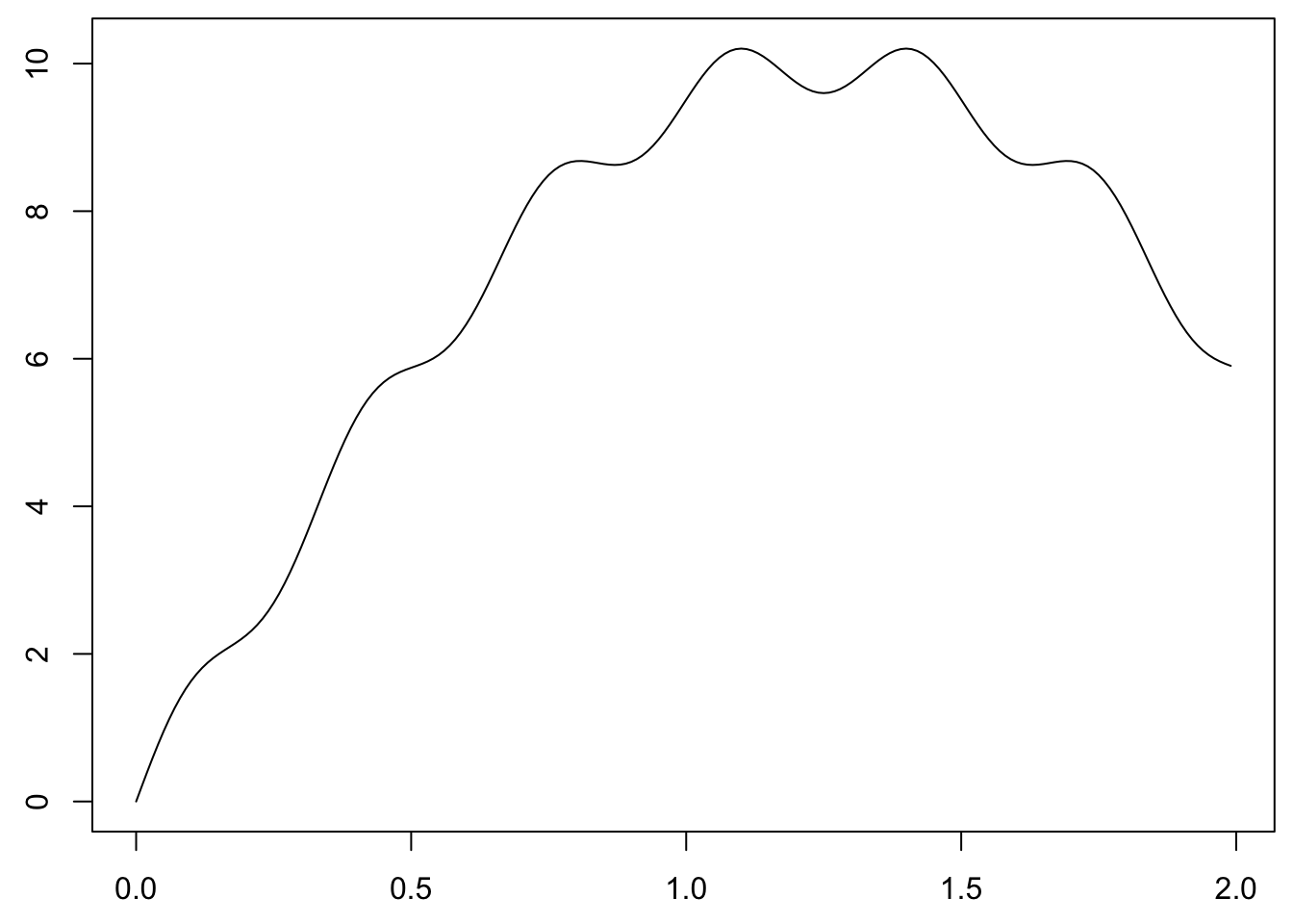
This section is an introduction to Fourier Analysis. We will cover a variety of topics including
How would you describe this signal?:
dt = 1/100
t = seq(from=0, by=dt, length=200);
y1 = 10*sin(2*pi*.2*t)
y2 = .4*sin(2*pi* 3*t);
y3 = y1+ y2
par(mai=c(.5, .5, .1,.1) )
plot(t, y3, type='l', xlab='', ylab='')The signal can be represented as a sum of different sinusoids:
par(mfrow=c(3,1) )
par(mai=c(.5, .5, .1,.1) )
plot(t, y1, ylim=range(y3) , type='l', xlab='', ylab='')
plot(t, y2, ylim=range(y3), type='l', xlab='', ylab='')
plot(t, y3, ylim=range(y3), type='l', xlab='', ylab='')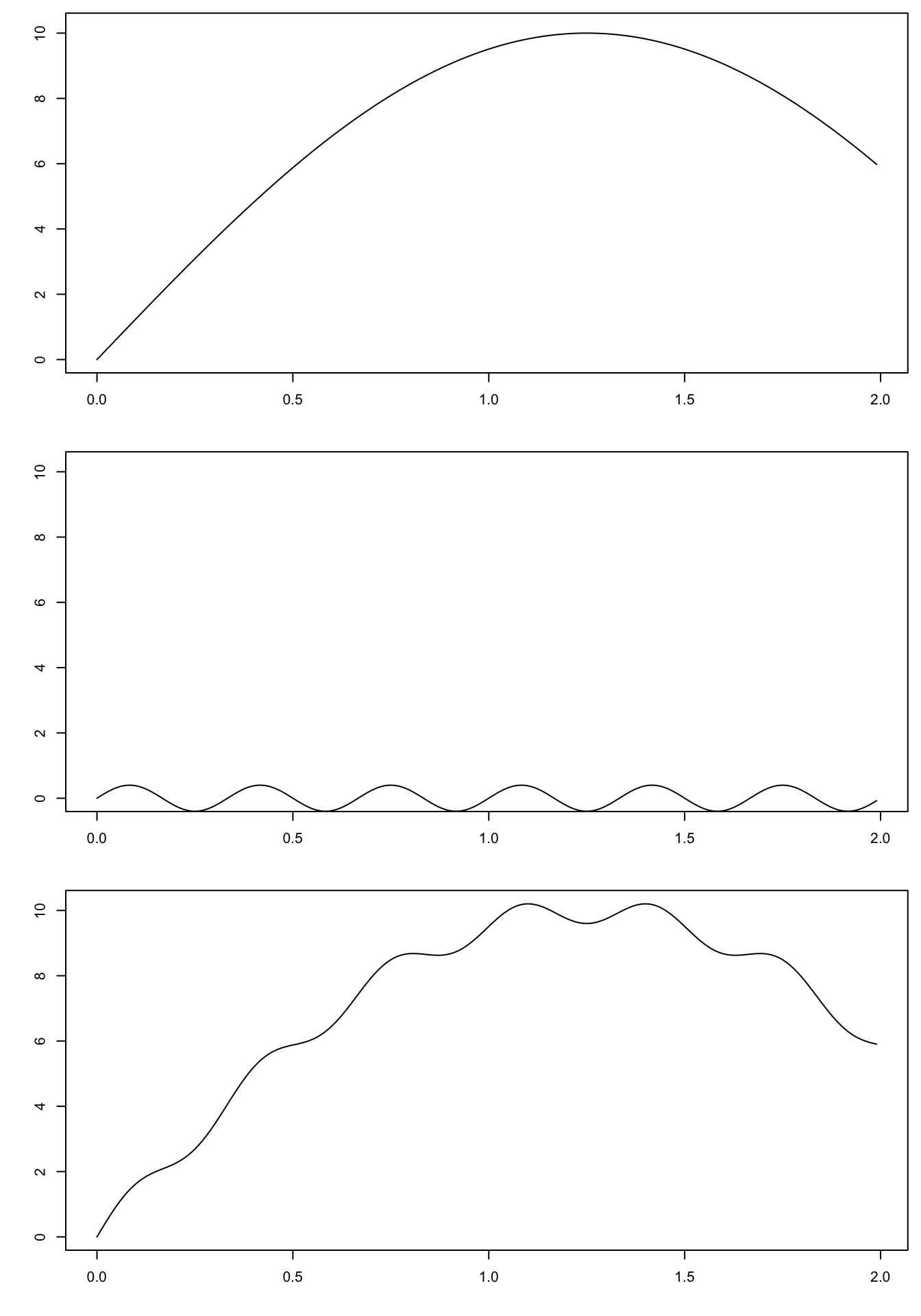
One could convey all the information with 6 numbers:
library(RSEIS)

dt = 0.001
omega = 4
A = 2
phi0 = 20*pi/180

x = seq(from=0, to=5, by=dt)
y = A*sin(omega*x - phi0)

aa <- which(peaks(y, span=3))

ay1 = y[aa[1]]+.1*A
ay2 = y[aa[2]]+.1*A

plot(range(x), range(y), type='n', ann=FALSE, axes=FALSE)
lines(x,y)
axis(1)
axis(2)

DT =0.2
g = seq(from=min(x), to=max(x), by=DT)
gy = A*sin(omega*g - phi0)

points(g,gy)
segments(g, rep(0, times=length(g)), g, gy, col=grey(0.85))
abline(h=0)


segments(x[aa[1]], ay1,x[aa[2]], ay2, lwd=2, col='red', xpd=TRUE)
segments(x[aa[1]], ay1,x[aa[1]],y[aa[1]] , col='red', xpd=TRUE)
segments(x[aa[2]], ay2,x[aa[2]],y[aa[2]] , col='red', xpd=TRUE)

segments(x[aa[3]], 0,x[aa[3]],y[aa[3]] , col='blue', lwd=2, xpd=TRUE)
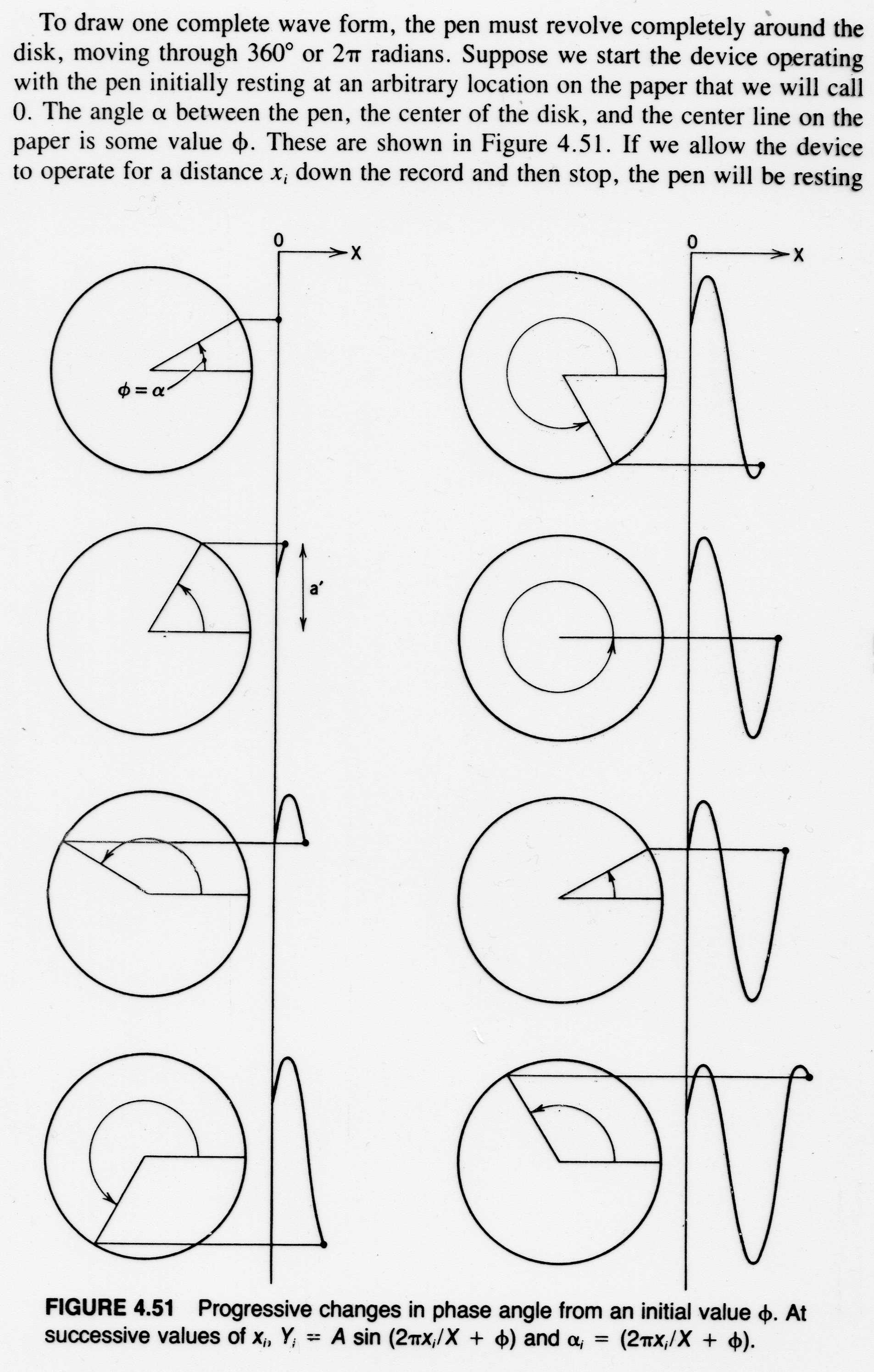
The rotating pen height in Figure 2.4 represents the signal. \[ Y_{i} = A \sin \left( 2 \pi x_{i}/X + \phi \right) \] \[ \alpha_{i} = \left( 2 \pi x_{i}/X + \phi \right) \]
Units:
if \(y = \cos ( \theta ) = \cos ( \omega t )\)
\[\begin{eqnarray*} y_{k} &=&A \cos(\omega t - \phi) \\ &=& A \cos (\omega t) \cos \phi + A \sin (\omega t) \sin \phi \\ &=& \alpha_{k} \cos (\omega t ) + \beta_{k} \sin(\omega t) \end{eqnarray*}\]
\[\begin{align*} \sin(u \pm v ) &= \sin u \cos v \pm \cos u \sin v \\ \cos ( u \pm v ) &= \cos u \cos v \mp \sin u \sin v\\ \end{align*}\]
Consider the Taylor series expansions:
\[\begin{eqnarray*} e^x &=& 1 + x +\frac{x^2}{2!}+\frac{x^3}{3!}+ \cdots \\ \sin(x) &=& x - \frac{x^3}{3!} + \frac{x^5}{5!} - \frac{x^7}{7!} + \cdots \\ \cos(x) &=& 1 - \frac{x^2}{2!} + \frac{x^4}{4!} - \frac{x^6}{6!} + \cdots \end{eqnarray*}\]
Plug in \(ix\) in the formula for \(e^x\) get: \[ e^{ix} = 1 + ix +\frac{(ix)^2}{2!}+\frac{(ix)^3}{3!}+\frac{(ix)^4}{4!}+\frac{(ix)^5}{5!}+\frac{(ix)^6}{6!}+\frac{(ix)^7}{7!}+\cdots \] Expanding out the complex numbers gives the trigonometric functions. \[ e^{ix} = \cos(x) + i \sin(x) \]
\[ e^{i\theta} = \cos(\theta) + i \sin(\theta) \] And \[ e^{-i\theta} = \cos(\theta) - i \sin(\theta) \] Add these together: \[ e^{i\theta} + e^{-i\theta} = 2 \cos(\theta) \] or: \[ \cos(\theta) = \frac{e^{i\theta} + e^{-i\theta}}{2} \] Similarly, by subtracting: \[ \sin(\theta) = \frac{e^{i\theta} - e^{-i\theta}}{2i} \]
\[\begin{eqnarray*} y_{k} &=&A \cos(\omega t - \phi) \\ &=& A \cos \omega t \cos \phi + A \sin \omega t \sin \phi \\ &=& \alpha_{k} \cos (\omega t ) + \beta_{k} \sin(\omega t) \end{eqnarray*}\]
The Fourier Coefficients are \(\alpha_{k} , \beta_{k}\)
This leads to Fourier’s Theorem: \[ Y = \sum_{k=0}^{\infty} A_{k} \cos(k\theta + \phi_{k}) \]
\[\begin{eqnarray*} \beta_{k} &=& \frac{2}{k}\sum_{j=0}^{n-1} Y_{j} \sin \left( \frac{2\pi j k}{n} \right) \\ \alpha_{k} &=& \frac{2}{k}\sum_{j=0}^{n-1} Y_{j} \cos \left( \frac{2\pi j k}{n} \right) \\ \end{eqnarray*}\]
The Zero-th value of the FT is the Mean value of the time series: \[ \alpha_{0} = \frac{1}{n} \sum_{j=0}^{n-1} Y_{j} \] This is usually called the DC or “direct current”.
Given the definition of the Fourier Series above, the spectrum is defined as: \[\begin{eqnarray*} A_{i} &=& \sqrt{a_{i} ^2 + b_{i} ^2} \\ \phi_{i} &=& \tan^{-1}\left( \frac{b_{i} }{a_{i} } \right) \end{eqnarray*}\]

if \(y = \cos( \theta ) = \cos( \omega t )\)
The Fourier transform of a function \(f(x)\) is a complex valued function \(F(\omega)\)
\[ FT(f) = F( \omega ) = \int_{-\infty}^{\infty} f(x) e^{- i x \omega } dx \]
Remembering that \(\omega = 2 \pi f\)
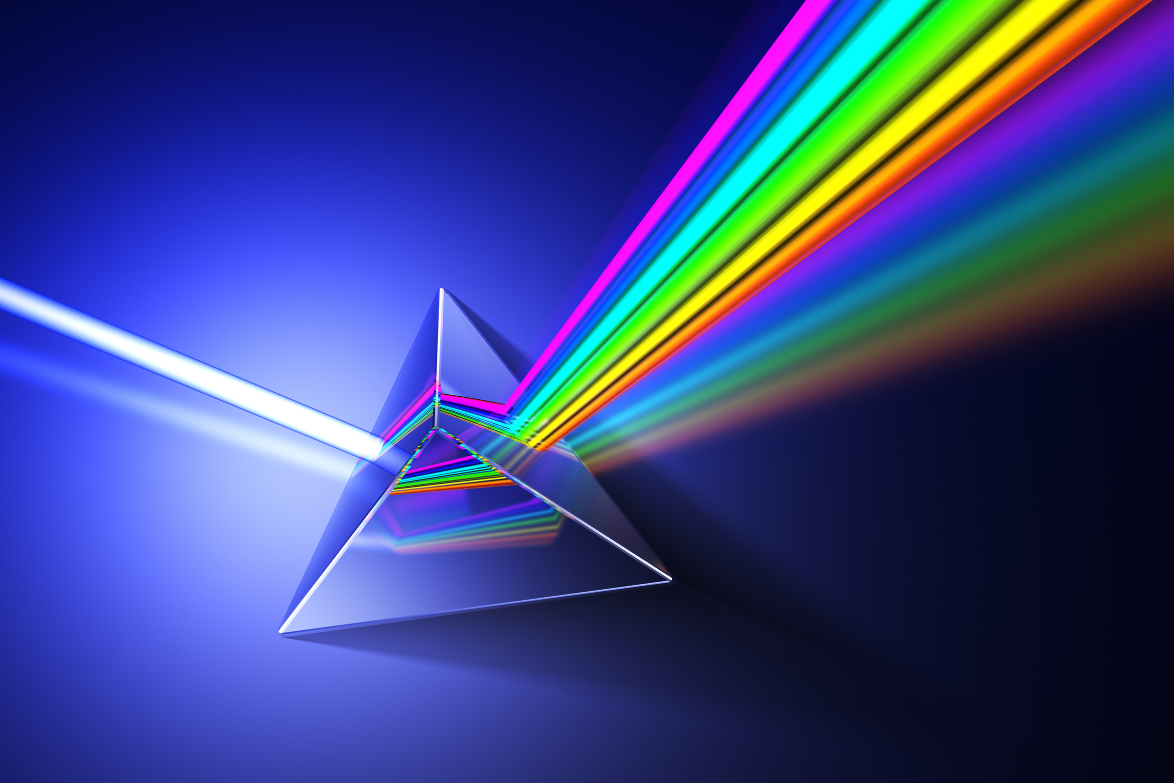
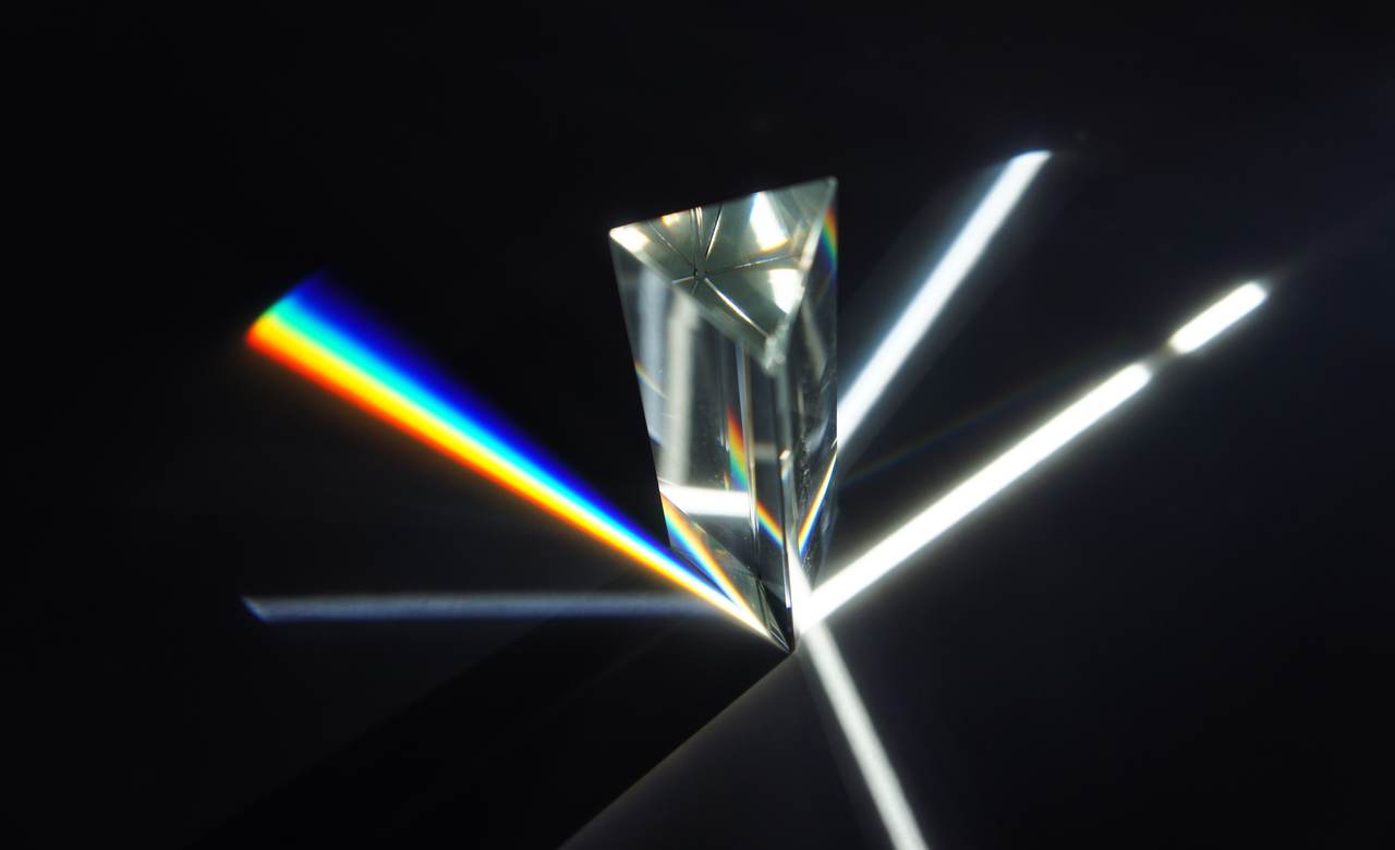
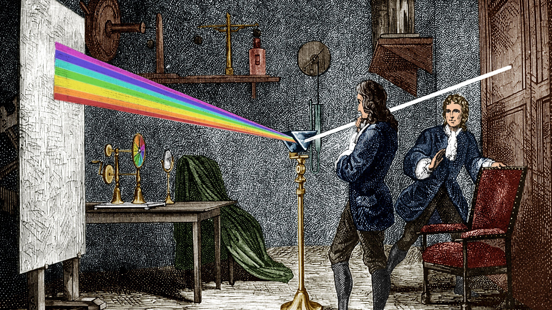
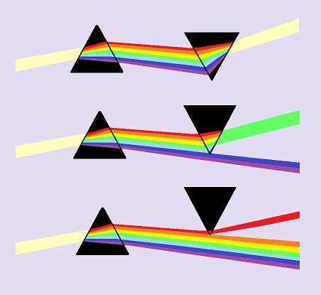
Think of the Fourier Transform like a prism: the input has numerous signals all combined: the FT separates the signals into sinusoidal elements and assigns a ‘power’, or level, to each component.
Suppose you have a time series, \(g\) that has \(n\) samples:
The Nyquist theorem states that we must sample an underlying signal at least twice per cycle in order to reconstruct a particular frequency. Or, if we sample at a rate of \(\Delta t\), then \[ f_{Nyquist} = \frac{1}{2\Delta t} \] is the maximum frequency we can extract without aliasing.
We can think of the amplitude spectrum is offering information on the statistical properties of the underlying time series: How much variance of the original signal is accounted for in each Fourier component?
This is the underlying concept of the Power Spectrum.
Convolution and Correlation of two time series are related:
\[ \left(f \star g\right)(t) \equiv \int_{-\infty}^{\infty} f^{\ast}(\tau)g(t+\tau) d\tau \]
To get the correlation: shift, multiply, sum
\[ \left(f \circledast g\right)(t) \equiv \int_{-\infty}^{\infty} f(\tau)g(t - \tau) d\tau \]
Shifting the time series multiplies the FT by a complex exponential.
\[ FT( g(x-a) ) = e^{-i \omega a} G(\omega) \]
Start with the definition of the FT: \(FT(g) = \int g e^{-i\omega t} dt\)
\[ \int_{-\infty}^{\infty} f(x-a) e^{- i 2 \pi x s}dx \]
Substitute \(u=x-a\), so that \(du=dx\) and \(x = u+a\):
\[ \int_{-\infty}^{\infty} f(u) e^{-i 2 \pi (u+a) s}du = \int_{-\infty}^{\infty} f(u) e^{-i 2 \pi u s} e^{-i 2 \pi a s} du = e^{-i 2 \pi a s} F(s) \]
Prove convolution theorem: \[ FT\left[ \int_{-\infty}^{\infty} f(\tau) g(t-\tau) d\tau \right] = F(\omega)G(\omega) \] Or, convolution in the time domain is multiplication in the frequency domain.
\[\begin{eqnarray*} FT\left[ \int_{-\infty}^{\infty} f(\tau) g(t-\tau)d\tau \right] &=& \\ \int_{-\infty}^{\infty} \int_{-\infty}^{\infty} f(\tau) g(t-\tau)e^{-i \omega t }d\tau dt &=& \\ \int_{-\infty}^{\infty} f(\tau) \int_{-\infty}^{\infty} g(t-\tau)e^{-i \omega t } dt d\tau &=& \\ \int_{-\infty}^{\infty} f(\tau) e^{-i \omega \tau } G(\omega) d\tau &=& F(\omega)G(\omega) \quad \square \end{eqnarray*}\]
Multiplication in the time domain is convolution in the frequency domain \[ g(t) \times f(t) \Leftrightarrow F(\omega) \circledast G(\omega) \] Multiplication in the frequency domain is convolution in the time domain \[ F(\omega) \times G(\omega) \Leftrightarrow g(t)\circledast f(t) \]
Example: Seismic Data

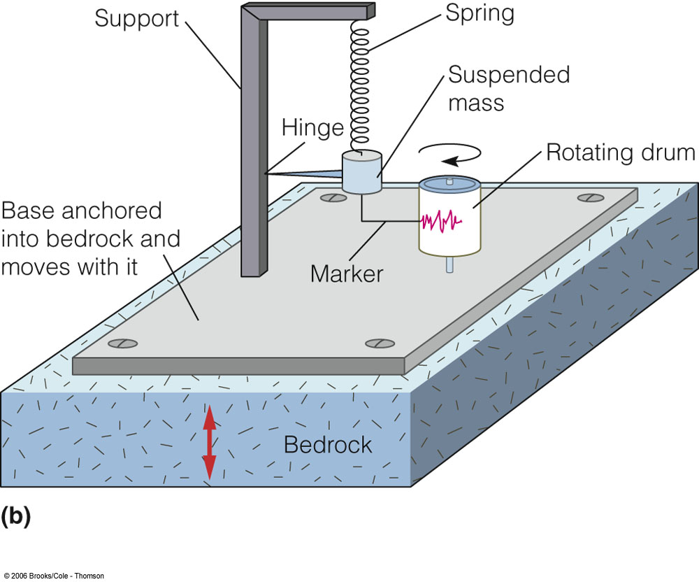
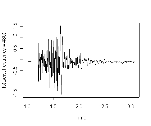
\[ Source ~~\bigotimes Earth ~~ \bigotimes ~~ Instrument ~~= ~~Signal \]
library(RSEIS)

dt = 0.01
freq = 16
nlen = 35

G = genrick(freq, dt, nlen)

tee = seq(from=0, by=dt, length=length(G))

x = sin(2*pi*freq*tee)*exp(-10*tee)

rx = rev(x)

mt1 = min(tee)
mt2 = max(tee)

x1 = min(x)
x2 = max(x)

rx1 = min(rx)
rx2 = max(rx)


spiks = rep(0, 50)
spiks[22] = 1
spiks[34] = 1

s1 = min(spiks)
s2 = max(spiks)

timesp = seq(from=0, by=dt, length=length(spiks))

st1 = min(timesp )
st2 = max(timesp )

c2 = convolve(x, spiks, type = c("open"))
ct = seq(from=0, by=dt, length=length(c2))
c21 = min(c2 )
c22 = max(c2 )

ct1 = min(ct)
ct2 = max(ct)

####
library(RPMG)

par(mai=c(.0, .0, .0,.0) )
plot(c(0,1), c(0,1.2), type='n', ann=FALSE, axes=FALSE)

lines(RESCALE(tee, 0, .4, mt1, mt2), RESCALE(x, 0.8, 1.0, x1, x2), col="blue")
text(0, 1.1, "Instrument Response", pos=4)


lines(RESCALE(timesp, .6, .9, st1, st2), RESCALE(spiks, 0.8, 1.0, s1, s2), col="blue")

text(0.6, 1.1, "Earth Response", pos=4)

lines(RESCALE(tee, 0, .4, mt1, mt2), RESCALE(rx, 0.5, .7, rx1, rx2), col="red")
text(0, 0.7, "Reversed Instrument Response", pos=4)

lines(RESCALE(timesp, .6, .9, st1, st2), RESCALE(spiks, 0.5, 0.7, s1, s2), col="blue")
arrows(.45, .6, .55, .6)

lines(RESCALE(ct, .2, .8, ct1, ct2), RESCALE(c2, 0.1, 0.3, c21, c22), col="purple")

text(.2 , 0.35, "Convolved Output", pos=4)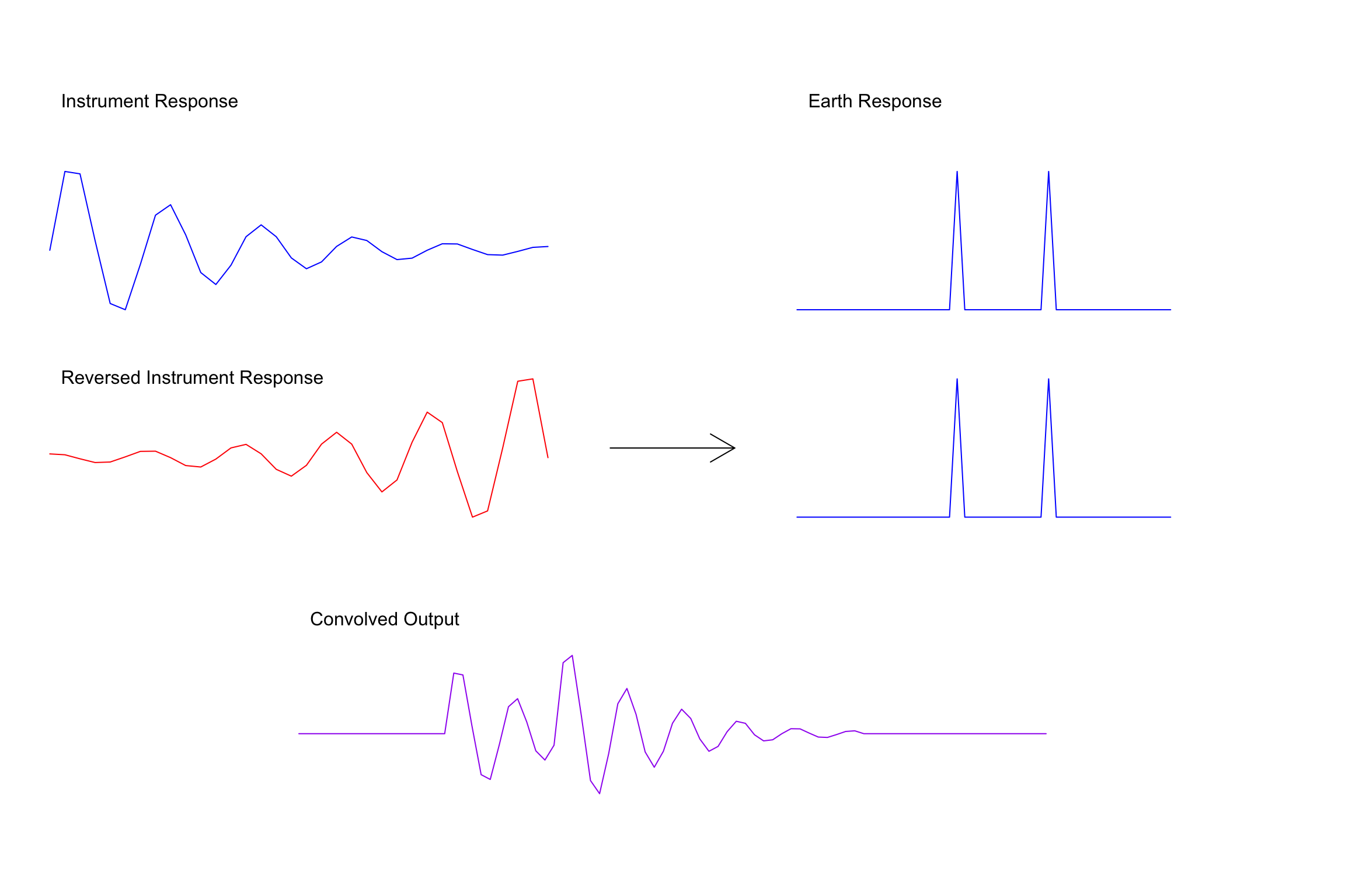
Convolution is the way processes interact in the earth. This is a model, of course, but it seems to work.
\[ C(t) = \int_{-\infty}^{\infty} A(t) B(-t) dt \]
Convolution is the cross correlation of one time series with the time-reversed version of another time series.
Recall the definition of the Autocorrelation: \[ Auto(\tau) = \frac{E\left[ (X_{t} - \mu ) (X_{t+\tau} - \mu) \right]}{\sigma^{2}} \] \[ FT\left[ \int_{-\infty}^{\infty} f(\tau) g(t+\tau)d\tau \right] = F(\omega)G^{\ast}(\omega) \] Let \(g=f\) in the convolution theorem, get Fourier Transform Autocorrelation: \[ FT\left[ \int_{-\infty}^{\infty} f(\tau) f(t+\tau)d\tau \right] = F(\omega)F^{\ast}(\omega) = \vert F(\omega) \vert^{2} \] This is commonly called the periodogram. It is a simple measure of the variance of each fourier component (sinusoid) represented in the signal.
The periodogram is not a good estimator of spectrum.
A standard measure of the similarity of a pair of signals is the coherency function defined by, \[ C(f) = \frac{S_1(f) \cdot S_2(f)} {\sqrt{S_1^2(f) S_2^2(f)} } \] where S1 and S2 are the complex Fourier transforms of the respective signals and (\(\cdot\)) is the dot product. In the case where we have multi-taper estimates of the spectra we can form the coherency function by using all n of the eigenspectra for each signal. In this case the coherence function is calculated by taking the inner vector product of the complex eigenspectra at each frequency, \[ C(f) = \frac{\sum_{k=1}^n S_{1k}(f) \cdot S_{2k}^{*}(f) }{ \sqrt{S_1^2(f) S_2^2(f)} } \] where * represents complex conjugation. The coherency function ranges from 0 to 1 and is measure of the coherency at each frequency.