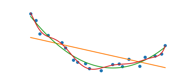
Numpy Polynomial Fitting

Given data out in the wild a common task is to fit a polynomial function. Numpy offers some convenient functions to get the job done.
%matplotlib inline
%config InlineBackend.figure_format = 'svg'

import numpy as np
import matplotlib.pyplot as plt
Generating data
We will create some mock data to explore polynomial fitting
# The unknown function we are trying to fit
f = lambda x: (x-3)**2

# Generating the sample points
x = np.linspace(0, 5, 20)

# Adding gaussian noise to x and f(x)
np.random.seed(123456)
noise_x = np.random.normal(0, .1, len(x))
noise_y = np.random.normal(0, .5, len(x))
data_x = x + noise_x
data_y = f(x) + noise_y
Let’s assume that this is our starting point. We are given some data and we wish to fit a polynomial. I always recommend plotting you data first!
plt.plot(data_x, data_y, 'o')
Now that we can see out data it’s time to fit!
Polynomial Fitting
The np.polyfit function is exactly what we want. Given a set of $xy$ points and a polynomial degree, np.polyfit returns the coefficients of the best fit. Lets see it in action
coeff = np.polyfit(data_x, data_y, deg=2)
print(coeff)
[ 0.94969091 -5.707748 8.46536612]
The coefficients are returned from highest to lowest power (note: The order of the coefficients is important). We can now use these coefficients to evaluate the polynomial.
# Polynomial Function
p2 = lambda x: coeff[0]*x**2 + coeff[1]*x + coeff[2]

# Points to evaluate
xp = np.linspace(min(data_x), max(data_x), 500)

# Plotting result
plt.plot(data_x, data_y, 'o')
plt.plot(xp, p2(xp), color='C2')
WAIT!!!
While what we have done has worked there is a flaw in our method. By handcrafting the polynomial function we have lost flexibility. If I want a 7th degree fit then we waste lots of time writing up a 7th degree polynomial function and introduce the possibility for errors. The np.poly1d function creates polynomial functions from the list of coefficients directly. Here the order matters and luckily np.poly1d expects the polynomial’s coefficients in decreasing powers which is exactly what np.polyfit returns. Lets create that 7th order polynomial fit
p7 = np.poly1d(np.polyfit(data_x, data_y,  7))
xp = np.linspace(min(data_x), max(data_x), 500)

plt.plot(data_x, data_y, 'o')
plt.plot(xp, p7(xp), color='C3')
Now we have a flexible procedure to do polynomial fitting. We can put this procedure into a loop and plot many polynomial fits
plt.plot(data_x, data_y, 'o')
xp = np.linspace(min(data_x), max(data_x), 500)
for degree in [1, 2, 10]:
    pn = np.poly1d(np.polyfit(data_x, data_y,  degree))
    plt.plot(xp, pn(xp), label='$p_{{{}}}$'.format(degree))
plt.legend()
There are many things one can do from here. Visualizing the error of the fit would be interesting, determining which fit is the best fit is important, but I will leave that for another post. Enjoy fitting polynomial to all of the things!